目录Contents
物理与统计:从零开始Physics and statistics: from zero
本页把项目用到的每个概念从零讲起,每个概念配一个算例。你只需要微积分、基础概率和入门 Python。
This page builds up every concept the project uses, from zero, each with a worked number example. You only need calculus, basic probability, and beginner Python.
1. 从光子到计数:有效面积与响应1. From photons to counts: effective area and response
XMM-Newton 的 EPIC-MOS 相机每 2.5 秒把天空拍一张「能量影像」:每个光子按到达的像素与能量(以通道号记录)登记。天文学家拿到的谱(spectrum,obj.pi 文件)是每能量通道的计数,不是能量流量。把「每秒每平方厘米的光子数」换算成「每通道计数」需要两件东西:
The EPIC-MOS cameras on XMM-Newton take an "energy image" of the sky every 2.5 s: each photon is logged by the pixel it hits and its energy (recorded as a channel number). The spectrum an astronomer gets (obj.pi) is counts per energy channel, not energy flux. Converting "photons per second per cm²" into "counts per channel" needs two things:
- 有效面积(effective area, ARF):望远镜+探测器对一个光子的「接住概率 × 面积」。MOS 在 1 keV 约为 400 cm²(峰值约 0.9 keV 处更高),在 2 keV 已明显下降。Effective area (ARF): the telescope+detector's "catch probability × area" for a photon. MOS is about 400 cm² at 1 keV (higher near the 0.9 keV peak) and clearly falling by 2 keV.
- 能量响应(response matrix, RMF):能量 E 的光子落在通道 c 的概率(高斯型展宽 + 探测边沿效应)。Response matrix (RMF): the probability that a photon of energy E lands in channel c (Gaussian-like broadening plus detector-edge effects).
算例:一个源每秒每平方厘米发出 1e-4 个 1 keV 光子,MOS 有效面积 400 cm²,曝光 10 ks(10⁴ s),探测效率约 0.9:预期计数 = 1e-4 × 400 × 1e4 × 0.9 ≈ 360 个。真实分析中由软件(Sherpa 的 RSP)自动完成这一乘法。
Worked example: a source emits 1e-4 photons s⁻¹ cm⁻² at 1 keV; the MOS effective area is 400 cm², the exposure is 10 ks (10⁴ s), and the detection efficiency is about 0.9: expected counts = 1e-4 × 400 × 1e4 × 0.9 ≈ 360 counts. In the real analysis this multiplication is done by the software (Sherpa's RSP).
来源:概念与数值为教科书常识(XMM-Newton Users' Handbook 的 MOS 有效面积量级);项目中的 ARF/RMF 文件见 data/0800730201/rpc/4.background/...(m31_cgmsum_v19_observation_products.csv 记录了每个场的 ARF/RMF 路径)。
Source: the concepts and scales are textbook standard (MOS effective-area order of magnitude from the XMM-Newton Users' Handbook); the project's ARF/RMF files live under data/0800730201/rpc/4.background/... and are listed per field in m31_cgmsum_v19_observation_products.csv.
2. 背景的四个来源2. The four sources of background
| 背景Background | 是什么What it is | 怎么处理How it is handled |
|---|---|---|
| QPB(准粒子背景)QPB (quiescent particle background) | 高能宇宙线/粒子在 CCD 里留下的电荷,与天空无关charge deposited in the CCD by high-energy cosmic rays/particles; nothing to do with the sky | 用视场外角区(corner)事件构的 back.pi 直接减掉(ESAS 方法)built into back.pi from out-of-field corner events and subtracted directly (the ESAS method) |
| SP(软质子)SP (soft protons) | 被磁场聚焦的小质子,随时变亮变暗(耀斑),谱近似幂律small protons focused by the magnetosphere, flaring on all timescales; spectrum approximately a power law | 逐谱拟合一个折断幂律(BreakE=3.2 冻结),norm 自由fitted per spectrum as a broken power law (BreakE=3.2 frozen), norm free |
| CXB(河外 X 射线背景)CXB (cosmic X-ray background) | 远处未分辨的 AGN 与星系,幂律 Γ≈1.46distant unresolved AGN and galaxies; a power law with Γ≈1.46 | 共享幂律分量,norm 自由a shared power-law component, norm free |
| LHB + 仪器线instr. lines | 太阳邻域 0.1 keV 热泡;MOS 的 Al/Si 荧光线(1.49/1.75 keV)the 0.1 keV solar-neighbourhood bubble; the MOS Al/Si fluorescence lines (1.49/1.75 keV) | LHB 共享拟合;仪器线逐探测器拟合,1.4–2.0 keV 整段剔除以免污染LHB fitted shared; instrumental lines fitted per detector, and the whole 1.4–2.0 keV band is excluded to avoid contamination |
另有 SWCX(太阳风电荷交换):太阳风的离子抢走中性氢的电子,发出线状软 X 射线——它随太阳风强度变化,是「时间性」背景,v19 里它的线分量(O7/O8/FeL)冻结为 0。E014 用 OMNI 太阳风数据检验了它:外 NW 四场的观测窗口无一超过 4e8 cm⁻² s⁻¹ 阈值,SWCX 作为解释被排除(D49)。
There is also SWCX (solar-wind charge exchange): solar-wind ions steal electrons from neutral hydrogen and emit line-like soft X-rays — a background that varies with the solar wind. v19 freezes its line components (O7/O8/FeL) at 0. E014 tested it with OMNI solar-wind data: no outer-NW window exceeded the 4e8 cm⁻² s⁻¹ threshold, so SWCX is excluded as the explanation (D49).
来源:处理方式依据 background_spectrum_fitting_2T_basedon_obsid_v19.py(模型与冻结状态见 design.html 表);SWCX 检验结论依据 cognition-os/experiments/E014(OMNI 节)与 cognition-os/04_DECISION_LOG.md D49。
Source: the handling follows background_spectrum_fitting_2T_basedon_obsid_v19.py (model and frozen states in the design.html table); the SWCX test result from cognition-os/experiments/E014 (OMNI section) and cognition-os/04_DECISION_LOG.md D49.
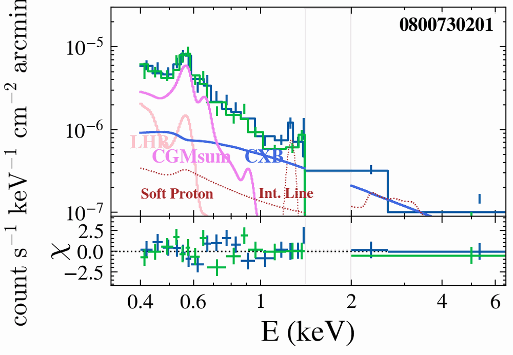
来源:background_spectrum_fitting_2T_basedon_obsid_v19_mos14to20keV_excluded_hi4pi_nh_per_pointing/0800730201_spectrum_fitting_1col.png(复制并压缩)。
Source: background_spectrum_fitting_2T_basedon_obsid_v19_mos14to20keV_excluded_hi4pi_nh_per_pointing/0800730201_spectrum_fitting_1col.png (copied and compressed).
3. 0.175 keV 热等离子体谱:kT 与 norm(emission measure)3. The 0.175 keV thermal plasma spectrum: kT and norm (emission measure)
一锅达到碰撞电离平衡的热气体发出轫致辐射连续谱 + 金属线。软件模型 APEC 用温度 kT(单位 keV;1 keV 对应 1.16×10⁷ K)与金属丰度 Z(相对太阳丰度)生成谱形。归一化(norm)定义为:
A hot gas in collisional ionisation equilibrium emits bremsstrahlung continuum + metal lines. The software model APEC builds the spectral shape from the temperature kT (in keV; 1 keV corresponds to 1.16×10⁷ K) and the metal abundance Z (relative to solar). The normalisation (norm) is defined as:
norm = (1 / (4π × D²)) × ∫ n_e n_H dV ≈ 1e-14 × EM / D_kpc² (with EM in cm^-3 pc)其中 ∫n_e n_H dV 是发射量(emission measure, EM),n_e 与 n_H 是电子与氢的数密度,D 是距离。算例:v19 里 0800730201 的 MWhalo norm ≈ 5.31e-6(每 arcmin²,见 byhand.html 命令 2)。反推其视线发射量:模型里 norm 已乘 skyarea(358.79 arcmin² = 1.033e-6 sr),对 D=785 kpc 的一条视线,EM ≈ norm × 4π D² / 1e-14 /(sr 换算)——量级为 10⁵ pc cm⁻³(一条 10 kpc 长的均匀视线对应 n_e ≈ 3×10⁻³ cm⁻³,正是 CGM 预期的密度)。
where ∫n_e n_H dV is the emission measure (EM), n_e and n_H are the electron and hydrogen number densities, and D is the distance. Worked example: in v19, 0800730201's MWhalo norm is about 5.31e-6 (per arcmin²; see command 2 on the by-hand page). Inverting to a line-of-sight emission measure: in the model the norm is already multiplied by skyarea (358.79 arcmin² = 1.033e-6 sr), so for a sightline at D = 785 kpc the EM is of order 10⁵ pc cm⁻³ (from norm × 4πD² / 1e-14 with the sr conversion) — for a uniform 10-kpc path that means n_e ≈ 3×10⁻³ cm⁻³, exactly the density expected for a CGM.
为什么是 0.175 keV?这个温度下气体主要在 O VII(0.57 keV)与 O VIII(0.65 keV)发出线,加上 Fe/Mg 的低能复合峰——恰好落在 MOS 最灵敏的 0.4–1.4 keV 窗口。温度再高(≥0.5 keV)线变弱;再低(≤0.1 keV)就出了 MOS 的下限。
Why 0.175 keV? At this temperature the gas radiates mainly in O VII (0.57 keV) and O VIII (0.65 keV) lines plus the low-energy Fe/Mg recombination bump — right in MOS's most sensitive 0.4–1.4 keV window. Hotter gas (≥0.5 keV) has weaker lines; colder gas (≤0.1 keV) falls below the MOS lower bound.
来源:norm 定义为 XSPEC APEC 标准;0800730201 的 norm 5.30805e-06 与 skyarea 358.79 来自 independent_cgm_v19_primary_dual_mos_measurements.csv;kT=0.17531±0.00436 来自 I012。EM 换算是本页的算例(建议(未经评审):核对时用 v19 脚本的 skyarea 定义)。
Source: the norm definition is the XSPEC APEC standard; 0800730201's norm 5.30805e-06 and skyarea 358.79 from independent_cgm_v19_primary_dual_mos_measurements.csv; kT=0.17531±0.00436 from I012. The EM conversion is this page's worked example (Suggestion (not reviewed): re-check with the v19 script's skyarea definition).
4. 银河系 HI 吸收(N_H)4. Absorption by Galactic HI (N_H)
X 射线穿过银河系盘的中性氢会被光电吸收,截面随能量下降(约 E⁻³):低能光子被吃掉得多。模型 XSphabs 用一列 N_H(单位 1e22 cm⁻²)描述。M31 方向的 N_H 取自 HI4PI 巡天(21 cm 全天图):对每个指向取 15 arcmin 孔径平均,范围 4.81e20–7.64e20 cm⁻²(即 0.048–0.076 × 1e22)。算例:N_H=0.058 × 1e22 时,0.5 keV 光子透过率约 0.4,1 keV 约 0.85,2 keV 约 0.95——所以 0.5–2 keV 流量是「吸收后」的,比固有值低两到三成(项目报告的就是这种吸收流量,单位注明 absorbed)。
X-rays crossing the Milky Way disc's neutral hydrogen are photoelectrically absorbed, with a cross-section falling roughly as E⁻³: low-energy photons are eaten first. The model XSphabs describes this with a column N_H (in 1e22 cm⁻²). Toward M31 the column comes from the HI4PI survey (an all-sky 21-cm map): a 15-arcmin aperture mean per pointing, spanning 4.81e20–7.64e20 cm⁻² (i.e. 0.048–0.076 × 1e22). Worked example: at N_H = 0.058 × 1e22, a 0.5 keV photon has transmission about 0.4, 1 keV about 0.85, 2 keV about 0.95 — so a 0.5–2 keV flux is "absorbed", two to three tenths below the intrinsic value (the project reports absorbed fluxes and labels them so).
来源:N_H 范围与孔径来自 cognition-os/experiments/E003「HI4PI QC」与 03_TRUST_TABLE.md「Per-OBSID HI4PI nH」;透过率数量级为标准光电截面(vern)的性质。
Source: the N_H range and aperture from cognition-os/experiments/E003 "HI4PI QC" and 03_TRUST_TABLE.md "Per-OBSID HI4PI nH"; the transmission scale follows the standard (vern) photoelectric cross-sections.
5. 表面亮度单位5. Surface-brightness units
弥漫发射的「亮度」是每单位天空面积的流量,本项目统一用 10⁻¹⁵ erg cm⁻² s⁻¹ arcmin⁻²。一个 XMM 场(有效提取面积约 350 arcmin²)的积分流量 ≈ 0.965 × 350 ≈ 3.4×10⁻¹³ erg cm⁻² s⁻¹——这就是「每场每秒穿过每平方厘米约 0.2 个光子」的量级。算例:14 场的逆方差平均 0.965 ± 0.044,意思是把 14 个测量按 1/σ² 加权平均后,统计误差约 4.5%(局部协方差误差,不含系统)。
The "brightness" of diffuse emission is flux per unit sky area; this project uses 10⁻¹⁵ erg cm⁻² s⁻¹ arcmin⁻¹ throughout. The integrated flux of one XMM field (effective extraction area about 350 arcmin²) is ≈ 0.965 × 350 ≈ 3.4×10⁻¹³ erg cm⁻² s⁻¹ — of order "0.2 photons per second per cm² per field". Worked example: the 14-field inverse-variance mean 0.965 ± 0.044 means that after weighting the 14 measurements by 1/σ², the statistical error is about 4.5% (local-covariance errors, no systematics included).
来源:0.965 ± 0.044 来自 I033;skyarea 例子(358.79 arcmin²)来自 independent_cgm_v19_primary_dual_mos_measurements.csv 的 0800730201 行。
Source: 0.965 ± 0.044 from I033; the skyarea example (358.79 arcmin²) from the 0800730201 row of independent_cgm_v19_primary_dual_mos_measurements.csv.
6. 为什么 MW 与 M31 谱形相同——只有空间形状能分辨6. Why MW and M31 spectra are identical — only spatial shape separates them
两条视线上的气体(银河系晕、M31 晕)如果 kT、Z、吸收都一样,APEC 谱逐通道相同——谱拟合无法把它们拆开。唯一的谱学线索是速度:M31 以约 −300 km/s 相对银河系运动,把 0.574 keV 的 O VII 线移动 ΔE = E × v/c ≈ 0.574 × 300/3e5 ≈ 0.0006 keV = 0.6 eV;而 MOS 在该能量的分辨率约 50 eV。所以「红移」完全测不出来(I006)。算例:把 MOS 分辨率想成一把 5 厘米刻度的尺子去量 0.6 毫米的差别——差 80 倍。
If the gas along two sightlines (the MW halo, the M31 halo) shares kT, Z and absorption, the APEC spectra are identical channel by channel — spectral fitting cannot split them. The only spectroscopic handle is velocity: M31 moves at about −300 km/s relative to the Milky Way, shifting the 0.574 keV O VII line by ΔE = E × v/c ≈ 0.574 × 300/3e5 ≈ 0.0006 keV = 0.6 eV, while MOS resolves about 50 eV there. The "redshift" is therefore unmeasurable (I006). Worked example: measuring a 0.6 mm difference with a ruler marked in 5 cm steps — a factor of 80 off.
剩下的判别信息是空间:M31 分量应随到 M31 的半径按 β 模型衰减;银河系分量应随银纬 b 缓慢变化(越靠银盘越亮)。14 个场沿短轴分布,恰好让「半径」与「纬度」在北侧共线、南侧反相——所以南北两侧的斜率符号能分离两种模型(I033 第 7 条)。注意:I033 曾据 Δχ²=6.2(≈2.5σ)把「纬度梯度」列为外 NW 四场偏亮的最佳假设;E014 用独立历元(RASS)与独立通道(OMNI 太阳风)检验后,大尺度纬度结构与 SWCX 都被排除,D49 改记为未解释场级系统误差。
The remaining discriminating information is spatial: an M31 component should decline with radius from M31 following a beta model, while the MW component should vary slowly with Galactic latitude b (brighter toward the plane). The 14 fields lie along the minor axis, so radius and latitude are nearly collinear on the north side and anti-correlated on the south — the slope signs on the two sides separate the two models (I033 item 7). Note: I033 once listed the "latitude gradient" as the best hypothesis for the bright outer-NW four from Δχ²=6.2 (≈2.5σ); after E014 tested it against an independent epoch (RASS) and an independent channel (OMNI solar wind), both large-scale latitude structure and SWCX were excluded, and D49 now carries it as an unexplained field-level systematic.
来源:cognition-os/insights/I006(0.6 eV vs 50 eV、五条出路);几何论证来自 cognition-os/insights/I033 第 7 条;E014 检验与 D49 结论见 cognition-os/experiments/E014 与 cognition-os/04_DECISION_LOG.md D49。
Source: cognition-os/insights/I006 (0.6 eV vs 50 eV and the five escape routes); the geometry argument from cognition-os/insights/I033 item 7; the E014 test and the D49 conclusion from cognition-os/experiments/E014 and cognition-os/04_DECISION_LOG.md D49.
7. β 模型:从 10 到 30 kpc 亮度掉多少7. The beta model: how much does the brightness fall from 10 to 30 kpc
等温气体球的投影亮度常用 β 模型:
The projected brightness of an isothermal gas sphere is usually written as a beta model:
S(r) = S_0 × (1 + (r/r_c)²)^(-3β + 1/2)r_c 是核半径(亮度开始下降的尺度),β 控制陡峭程度。算例(与 I033 一致,r_c=4 kpc,在 R=20 kpc 归一):
r_c is the core radius (the scale where the brightness starts to fall) and β sets the steepness. Worked example (matching I033, r_c = 4 kpc, normalised at R = 20 kpc):
β=0.4: S(10.5)/S(20) = ((1+(20/4)²)/(1+(10.5/4)²))^0.3 = (26/7.89)^0.3 ≈ 2.6   → falls by 3.8× from 10.5 to 29 kpc
β=0.5: exponent 1.0   → falls by 6.8×
β=0.6: exponent 1.3   → falls by 12.1×
但 14 个场的数据没有显示这种下降(χ²=11.99/13 的常数拟合已足够)。如果 M31 分量真是 r_c=4 kpc 的 β 模型,它最多只能贡献总量的 10–20%(MW 常数版 0.05–0.12 @20 kpc,D49 后默认;MW 线性 b 版 0.08–0.19 所依赖的纬度梯度已被 E014 排除)。
But the 14 fields show no such decline (a constant fit with χ²=11.99/13 is already adequate). If the M31 component really were a beta model with r_c=4 kpc, it could contribute at most 10–20% of the total (the MW-constant version gives 0.05–0.12 at 20 kpc, the default after D49; the MW linear-in-b version, 0.08–0.19, relied on the latitude gradient that E014 excluded).
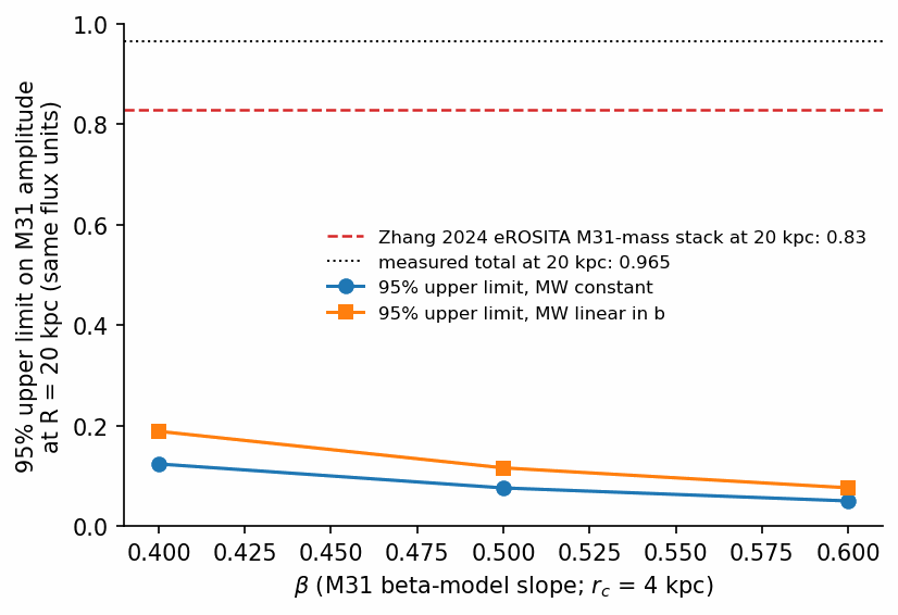
数据:newangels3_discussion/quick_beta_amplitude_limits_20261014.csv(β=0.4/0.5/0.6,r_c=4 kpc);Zhang 0.828 来自 paper_apj_v19_cgmsum_draft/data/m31_cgmsum_conditional_prior_ledger.csv(zhang2024_m31_mass_nominal_20kpc 行)。图由 handbook/hermes_figscripts/make_figures.py 生成。
Data: newangels3_discussion/quick_beta_amplitude_limits_20261014.csv (β=0.4/0.5/0.6, r_c=4 kpc); Zhang 0.828 from paper_apj_v19_cgmsum_draft/data/m31_cgmsum_conditional_prior_ledger.csv (the zhang2024_m31_mass_nominal_20kpc row). Figure made by handbook/hermes_figscripts/make_figures.py.
8. χ²、profile likelihood 与单侧上限8. Chi-square, profile likelihood, and one-sided upper limits
χ² 检验:把数据分箱后,χ² = Σ (观测 − 模型)²/σ²。自由度 dof = 箱数 − 自由参数数。「χ²/dof ≈ 1」表示模型与数据涨落一致。例如常数拟合 14 个场:χ² = 11.99,dof = 13,p = 0.53——一个常数完全够用,不需要径向趋势。
The chi-square test: after binning, χ² = Σ (observed − model)²/σ². The degrees of freedom are dof = (number of bins) − (number of free parameters). "χ²/dof ≈ 1" means the model is consistent with the data scatter. For the 14-field constant fit: χ² = 11.99, dof = 13, p = 0.53 — a constant is fully adequate; no radial trend is needed.
Δχ² / Δstat 比较:两个嵌套模型,多一个参数通常把 χ² 降低约 1(无信息时)。线性银纬模型把 χ² 从 11.99 降到 5.77,Δχ² = 6.2——单参数改善 6.2,对应约 2.5σ(χ²(1) 的 p ≈ 0.013)。线性半径只有 Δχ² = 3.7(1.9σ)。所以「银纬」比「半径」更受数据支持,但都不到 3σ;而 E014 的独立检验(RASS、OMNI)没有复现这个梯度,D49 已把它改记为未解释场级系统误差。
Δχ² / Δstat comparison: for two nested models, one extra parameter typically lowers χ² by about 1 (when it carries no information). The linear-in-latitude model drops χ² from 11.99 to 5.77, Δχ² = 6.2 — a one-parameter improvement of 6.2, about 2.5σ (χ²(1) p ≈ 0.013). Linear-in-radius gives only Δχ² = 3.7 (1.9σ). So "latitude" is favoured over "radius", but neither reaches 3σ; and E014's independent tests (RASS, OMNI) did not reproduce the gradient, so D49 now carries it as an unexplained field-level systematic.
Profile likelihood 与边界:想知道「M31 幅度 A 是多少」时,固定 A,把其余所有参数重新最优,得到 stat(A) 曲线;A 的 68% 区间是 stat 上升 1 的范围(1 自由度的 Δstat=1 规则)。麻烦在 A 的物理下界是 0:如果最佳拟合就在 A=0 附近或以下,普通 χ² 区间会算出负的 A。正确做法是单侧上限:A < A_95,其中 A_95 用 Δstat = 2.71(1 自由度 95% 单侧)或用模拟校准覆盖率得到。这正是 I008 的 U0/U1/U2 阶梯与 E013 A2 的设计。
Profile likelihood and the boundary: to ask "what is the M31 amplitude A", freeze A, re-optimise everything else, and get the stat(A) curve; the 68% interval is where stat rises by 1 (the Δstat=1 rule for one degree of freedom). The trouble is that A's physical lower bound is 0: if the best fit sits at or below A=0, an ordinary chi-square interval produces negative A. The correct tool is a one-sided upper limit: A < A_95, with A_95 from Δstat = 2.71 (one-parameter one-sided 95%) or from simulation-calibrated coverage. That is exactly the U0/U1/U2 ladder of I008 and the design of E013 A2.
算例:β=0.5、MW 常数时,A20 的拟合中心是 −0.074 ± 0.046(负值,即无需 M31 分量);近似 95% 单侧上限 = max(0, −0.074) + 1.645 × 0.046 = 0.076(quick_beta_amplitude_limits_20261014.csv 的 β=0.5、mw_model=const 行)。
Worked example: for β=0.5 with the MW term constant, the fitted A20 centre is −0.074 ± 0.046 (negative — no M31 component needed); the approximate one-sided 95% upper limit is max(0, −0.074) + 1.645 × 0.046 = 0.076 (the β=0.5, mw_model=const row of quick_beta_amplitude_limits_20261014.csv).
来源:χ² 与 Δχ² 数值来自 newangels3_discussion/quick_shape_limit_20261014.txt 第 1–4 行;A20 与 1.645σ 上限来自 quick_beta_amplitude_limits_20261014.csv;profile/单侧上限原则来自 cognition-os/insights/I008「Required coverage definition」与 03_TRUST_TABLE.md D22 行;E014 未复现与 D49 改记见 cognition-os/experiments/E014 与 04_DECISION_LOG.md D49。
Source: the χ² and Δχ² numbers from newangels3_discussion/quick_shape_limit_20261014.txt lines 1–4; A20 and the 1.645σ limit from quick_beta_amplitude_limits_20261014.csv; the profile/one-sided-limit principles from cognition-os/insights/I008 "Required coverage definition" and the D22 row of 03_TRUST_TABLE.md; the E014 non-reproduction and the D49 reclassification from cognition-os/experiments/E014 and 04_DECISION_LOG.md D49.
9. 动画:β 模型滑块9. Animation: the beta-model sliders
下面这个交互图把 14 个测量点固定,让你拖 r_c、β 与 M31 幅度 A:总和保持为测量的 0.965(MW = 0.965 − A)。β 越大或 r_c 越小,M31 分量越向中心集中,χ² 越差——直观看到「为什么集中式 M31 晕最多只能占 10–20%」。
The interactive plot below pins the 14 measured points and lets you drag r_c, β and the M31 amplitude A; the total is held at the measured 0.965 (MW = 0.965 − A). Larger β or smaller r_c concentrates the M31 component toward the centre and worsens χ² — a direct feel for "why a concentrated M31 halo can be at most 10–20% of the total".